Network Analysis with R

This page is part of my final project for a network analysis course. While I don’t plan to develop it into a full paper at the moment, I think it’s a useful opportunity to practice network analysis and demonstrate how to run a latent space model in R. Although applying a latent space model to this research design and dataset has clear limitations, I hope readers see it primarily as a reference for how to draw a network plot and implement the model in R, rather than as a fully justified methodological choice.

Let’s get started!

First, load the required packages:

library(network)
library(sna)
library(latentnet)
library(viridis)
library(knitr)
library(kableExtra)
library(dplyr)
library(tidyverse)

Second, load the network dataset. You can download the dataset here

net <- readRDS("net.rds")

This dataset represents a network of countries that intervened in the same civil wars, with a focus on identifying patterns of collaboration among intervening states. Each node corresponds to a country, and a tie (or edge) is formed between two countries if they supported the same side—either the government or the rebels. To construct these dyads of co-intervening countries, I draw on the Uppsala Conflict Data Program (UCDP) External Support Dataset (ESD), which is structured as panel data. Each row in the ESD provides information on the recipient of external support, the external supporter, the opposing actor, and the year of the conflict. For analytical consistency, the analysis is limited to the year 2012—the most recent year for which complete data across all covariates are available.

To better capture the dynamics of co-intervention, the dataset includes covariates at both the node (country) and edge (dyadic) levels. At the country level, each node is annotated with regime type, derived from the Varieties of Democracy (V-Dem) dataset. The regime classification ranges from closed autocracy (value = 0), where there are no multiparty elections for either the chief executive or the legislature, electoral autocracies (value = 1), where multiparty elections exist but fail to meet standards of freedom or fairness, to electoral democracies (value = 2), which meet Dahl’s criteria for polyarchy but lack liberal institutional guarantees, and liberal democracies (value = 3), which uphold both electoral and liberal democratic standards, including civil liberties, rule of law, and executive accountability. Countries are also assigned to one of six geographical regions, as categorized by V-Dem: (1) Eastern Europe and Central Asia, (2) Latin America and the Caribbean, (3) the Middle East and North Africa, (4) Sub-Saharan Africa, (5) Western Europe and North America, and (6) Asia and the Pacific.

At the dyadic level, the dataset incorporates information on whether two countries are formal military allies, using data from the Correlates of War (COW) alliance dataset. It also captures whether both countries supported the government side in the same civil conflict, distinguishing such partnerships from those in which both supported rebel actors.

To visualize the network, I create a network plot using the dataset, with nodes colored by democracy level.

The first step is to assign a color to each country based on its level of democracy.

# Extract the names of the nodes (i.e., countries) from the network object
lab <- network.vertex.names(net)

# Get the unique values of the "Democracy1" attribute (which encodes regime types)
unique_polyarchy <- sort(unique(net %v% "Democracy1"))

# Generate a vector of distinct colors for each regime type using the 'viridis' palette
colors <- viridis(length(unique_polyarchy), option = "D")

# Define labels corresponding to each regime type
labels <- c("Closed Autocracy", "Electoral Autocracy", 
            "Electoral Democracy", "Liberal Democracy")

# Create a named color map where each regime type
# is associated with one of the generated colors
color_map = setNames(colors, unique_polyarchy)

# Assign a specific color to each node based on its regime type
node_colors <- color_map[as.character(net %v% "Democracy1")]

Since the dataset includes too many countries, plotting all of them would result in a cluttered and unreadable graph. So, I randomly selected 30 countries to include in the plot.

# Set a random seed for reproducibility.
# Ensures that the random sample drawn next is the same every time you run the code
set.seed(14)

# Randomly selects 30 countries for the network
selected_vertices <- sample(network.vertex.names(net), 30)

# Finds the indices (numeric positions) of the selected countries in the network.
vertex_ids <- which(network.vertex.names(net) %in% selected_vertices)

# Creates a subgraph that includes only the selected 30 countries and the connections among them.
net_sub <- get.inducedSubgraph(net, v = vertex_ids)

Now, let’s start drawing the plot!

# Splits the plotting window into two columns to display two plots side-by-side.
par(mfrow = c(1, 2))

# Plots the first sample of 30 countries.
# label = lab[vertex_ids] assigns country names as labels.
# vertex.col = node_colors[...] assigns node colors based on democracy level.
# mtext() adds the label "(a) Sample 1" below the plot.
plot(net_sub, label = lab[vertex_ids], vertex.col = node_colors[vertex_ids], edge.col = "gray", vertex.cex = 1, label.cex = 0.6)
mtext("(a) Sample 1", side = 1, line = 2, cex = 1.2)

# Repeats the above steps with a different random seed to generate a different subset of 30 countries.
set.seed(128)
selected_vertices1 <- sample(network.vertex.names(net), 30)
vertex_ids1 <- which(network.vertex.names(net) %in% selected_vertices1)
net_sub1 <- get.inducedSubgraph(net, v = vertex_ids1)
plot(net_sub1, label = lab[vertex_ids], vertex.col = node_colors[vertex_ids], edge.col = "gray", vertex.cex = 1, label.cex = 0.6)
mtext("(b) Sample 2", side = 1, line = 2, cex = 1.2)

# Resets the plotting window back to a single panel.
par(mfrow=c(1,1))

# Allows drawing outside the plot region - needed for the legend
par(xpd = NA)

# Adds a horizontal legend at the bottom of the plot.
# The legend shows the meaning of node colors (regime types).
# pch = 19 draws solid circle markers.
# bty = "n" removes the box around the legend.
legend("bottom", 
       inset = c(0, -0.25),  
       legend = labels, 
       col = color_map, 
       pch = 19, 
       pt.cex = 1,
       cex = 1,
       horiz = TRUE,
       bty = "n")

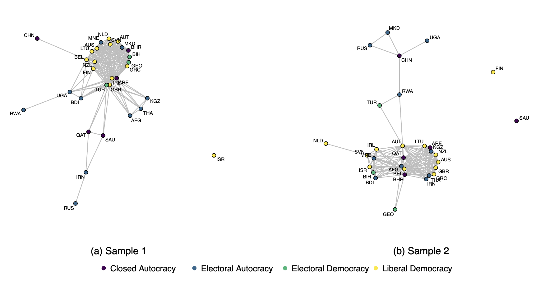
The plot shows sample networks of two sets of 30 randomly selected external supporters, colored by their level of democracy. Both samples illustrate that most liberal democracies tend to have more ties, whereas autocracies are connected to only a few countries.

To examine patterns of co-intervention among states in civil conflicts, I employ a Latent Space Model (LSM), a network model suited for analyzing relational data influenced by both observed covariates and unobserved structural dependencies. Latent space models are grounded in the assumption that dependencies in network data can be viewed as being the result of the distances between individuals in some social, physical, or other latent space, and that the likelihood of a tie is inversely related to the distance between nodes in this latent space.

The probability of an edge \( y_{ij} \) between the two nodes \( i \) and \( j \) in the network is modeled as:

$$ \text{logit}(\Pr(y_{ij} = 1)) = \eta_{ij} = \beta_0 + X_{ij} \beta - d(z_i, z_j) $$

Here, \( X_{ij} \) represents dyadic covariates, \( \beta \) is the vector of coefficients associated with the covariates, and \( d(z_i, z_j) \) is the Euclidean distance between the latent positions \( z_i \) and \( z_j \) in an unobserved social space.

model1 <- ergmm(net ~ euclidean(d=2), verbose = TRUE, seed=125)

This code estimates a baseline latent space model for your network, without covariates—just using latent distances to explain the presence of ties. It serves as a foundational model before adding node or dyadic covariates.

par(mfrow=c(1,2))
plot(model1, plot.vars=FALSE, pad=0,  vertex.col = node_colors)
plot(model1, what="pmean", plot.vars=FALSE, pad=0,  vertex.col = node_colors)

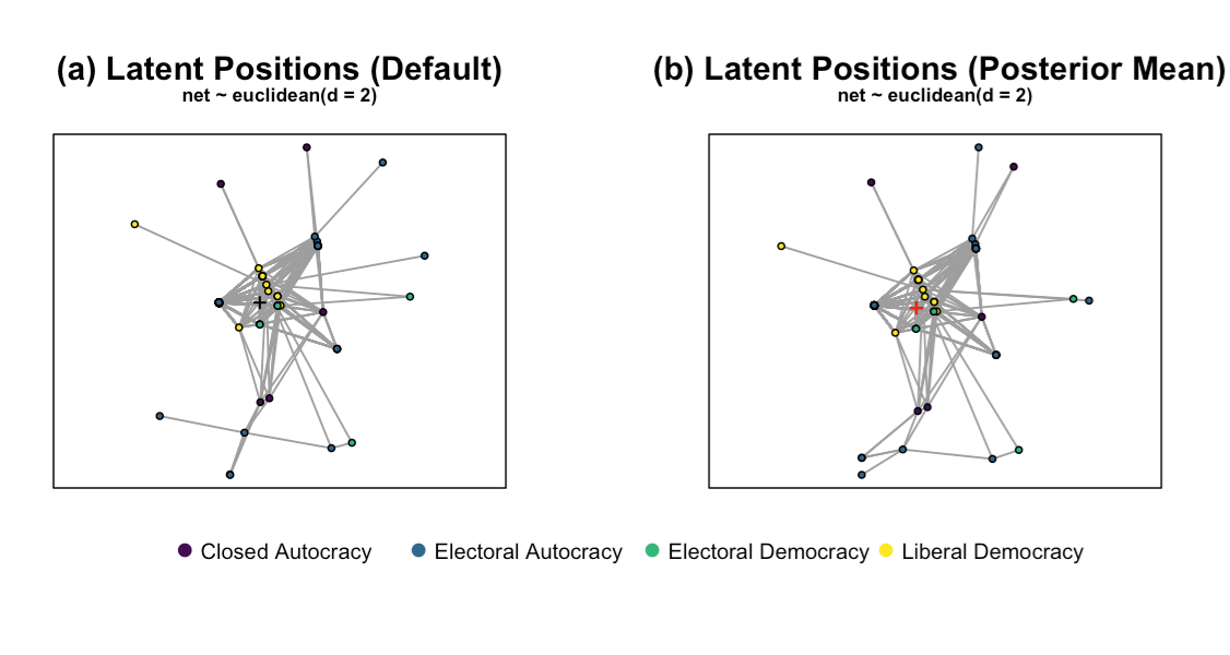
This code produces two side-by-side network plots based on your latent space model:

(Left): One sample of the latent space configuration.

(Right): The posterior mean of the latent positions.

Both plots help visualize how countries are positioned in latent space, with nodes colored by regime type.

Below is the model that includes the key explanatory variable: democracy level.

model2 <- ergmm(net ~ nodematch("Democracy1", diff= TRUE) + euclidean(d=2), control = control.ergmm(burnin=250000), seed=10, verbose= TRUE)

Now, I include the controls to the model:

model3 <- ergmm(net ~ nodematch("Democracy1", diff= TRUE) + nodematch("Region", diff=FALSE) + nodematch("Income_group", diff=TRUE) + edgecov(alliance) + edgecov(supportgov) + euclidean(d=2), control = control.ergmm(burnin=250000), seed=10, verbose= TRUE)

Let’s take a look at the results.

summary(model2)
summary(model3)

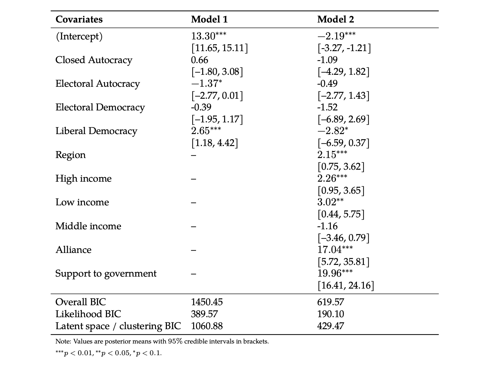
The table presents the posterior estimates from two latent space models analyzing the probability that states co-intervene in the same civil war. Both models are estimated using Bayesian techniques and account for latent proximity between states. Model 1 includes only the key independent variable of this research—regime-type indicators, while Model 2 adds a set of control variables to the basic model. In Model 1, the coefficient for Liberal Democracies exhibits a positive association with co-intervention (2.65), suggesting that countries are more likely to coordinate intervention efforts when both are liberal democracies. In contrast, Electoral Autocracies have a negative effect, indicating that countries are less likely to support the same actor in civil wars if both belong to that regime type. These results provide support for my hypotheses in the case of liberal democracies and electoral autocracies, showing that democratic countries are more likely to co-intervene in the same civil war dyad and often align on the same side, while autocracies are not. However, the coefficients for Electoral Democracies and Closed Autocracies are not statistically significant, indicating weaker evidence for these categories.

Model 2 tells a different story from Model 1. After controlling for additional covariates such as region, income group, and edge-level variables, the coefficient for Liberal Democracies becomes negative (–2.82), suggesting that the observed tendency of liberal democracies to co-intervene—seen in Model 1—is likely confounded by other factors. When those confounders are held constant, liberal democracies appear less likely to jointly intervene compared to other regime types. At the same time, Alliance Ties and Support to Government emerge as the main predictors of co-intervention. This indicates that countries that have formal alliances or common interests or support the government side over rebel groups are highly likely to intervene together, regardless of regime type.

In addition, Model 2 shows that regional proximity and shared high-income or low-income status all positively predict co-intervention. This suggests that countries with similar geographic or economic characteristics are more likely to coordinate intervention efforts, possibly due to overlapping security concerns, economic interests, or regional institutional frameworks. For the model fit, Model 2 outperforms Model 1 across all BIC metrics, indicating that the inclusion of region, income group, and edge-level covariates improves explanatory power.